Transformers Tutorial (In More Detail)
Transformers Tutorial (In More Detail)
In the tutorial, on the one hand we have the torchtext data and the other hand we are building a transformer model for NLP. The tutorial doesn't aim to produce a model that is useful except for seeing loss decreasing.
TorchText Data
TorchText data gives an iterator. Each element in the iterator is a line of text from wikipedia articles.
train_iter = WikiText2(split='train')
If we print out some of the items in the iterator, we get something to the following.
0

1  = Valkyria Chronicles III =

2

3  Senjō no Valkyria 3 : <unk> Chronicles ( Japanese : 戦場のヴァルキュリア3 , lit . Valkyria of the Battlefield 3 ) , commonly referred to as Valkyria Chronicles III outside Japan , is a tactical role @-@ playing video game developed by Sega and Media.Vision for the PlayStation Portable . Released in January 2011 in Japan , it is the third game in the Valkyria series . <unk> the same fusion of tactical and real @-@ time gameplay as its predecessors , the story runs parallel to the first game and follows the " Nameless " , a penal military unit serving the nation of Gallia during the Second Europan War who perform secret black operations and are pitted against the Imperial unit " <unk> Raven " .

4  The game began development in 2010 , carrying over a large portion of the work done on Valkyria Chronicles II . While it retained the standard features of the series , it also underwent multiple adjustments , such as making the game more <unk> for series newcomers . Character designer <unk> Honjou and composer Hitoshi Sakimoto both returned from previous entries , along with Valkyria Chronicles II director Takeshi Ozawa . A large team of writers handled the script . The game 's opening theme was sung by May 'n .
We get lines of text and we will have to process the text to use for learning.
The code for this is at https://github.com/mochan-b/pytorch-tutorial1/blob/main/torchtext_data.py
Transformer Model and PyTorch Implementation
Before we get started, just want to point out that word "encoder" is used in two different contexts in the original tutorial. We will just make sure the point it out to avoid confusion when using the word encoder.
Encoder Architecture
The original transformer architecture has an encoder-decoder architecture; left side called encoder and right side called decoder. It is possible to just use the encoder, decoder and encoder-decoder architecture. Obviously just from the pictures, the encoder part is the smallest and best suited for a tutorial.
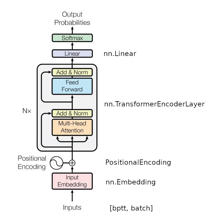
In the figure, we take the left side of the transformer encoder layer and then add the linear and softmax from the decoder layer. In this tutorial, we use nn.Embedding and nn.TransformerEncoderLayer from PyTorch but use our own PositionalEncoding. We are also responsible for creating the inputs from text.
Let's explore each of the layers in detail here.
Inputs
This will be the data from torchtext.
However, this is not straight up text. It has to be processed quite a bit before it can be become input and this is further discussed in section on creating the input data from torchtext below.
But the main idea is that input must be integers; where each number represents a token. A token can be a character, word or phrase and each is mapped to an integer. An unknown token is also given that is a bucket for anything that isn't in the corpus.
Input Embedding
We use nn.Embedding already defined in pytorch for this. Note that we call it with nn.Embedding(ntoken, d_model). ntoken is the number of tokens that is possible and d_model is the dimension of the output of the embedding.
Embeddings find a d_model-dimensional representation of a token. Two tokens who are closely related will have an embedding will be similar even though its indices might be completely different.
Positional Encoding
We roll our own positional encoding that is from the original transformer paper in the PositionalEncoding. You'd expect there to be nn.PositionalEncoding but its not there.
Even though we send the data in order, the architecture downstream processes all of the indices in parallel and so position information has to be encoded into the data itself.
It can be quite confusing when we see sines and cosines and just being added to the input data. There is some theory behind it but the important thing is that it adds the position information.
Technically, we could just add 0, 1, 2, ... to all of the data in front of the actual value. However, the sine and cosine version of position encoding works better while training in practice.
Transformer Encoder
TransformerEncoderLayer layer wraps up trident that copies the data into multi-head attention, does the add and normalization and feed-forward and add and norm into a class as in Figure for the transformer above above.
This takes in d_model which is the size of the features that comes out of the embedding layer.
The nhead is not represented in the original diagram but can imagine it extending into 3d. Basically we have the same head where the data goes in and are concatenated.
The feed-forward network has 2 layers and dim_feedforward determines the width of the network. dropout is the Dropout parameter used in various places between the various places.
As from the Nx in the transformer diagram, the layer is repeated. Here, nlayers is the parameter for it.
Linear (Decoder) Layer
This decoder is different than a transformer decoder but is a linear layer that takes an embedding sized output from the encoding-layer and produces a probability for each token.
Model
When printing the model we get the following. The TransformerEncoder is built up from MultiheadAttention that is unique to transformers and a combination of Linear, Dropout and LayerNorm.
All the features are from the tutorial except for the vocabulary size of 10,000.
TransformerModel(
(pos_encoder): PositionalEncoding(
(dropout): Dropout(p=0.2, inplace=False)
)
(transformer_encoder): TransformerEncoder(
(layers): ModuleList(
  (0-1): 2 x TransformerEncoderLayer(
    (self_attn): MultiheadAttention(
      (out_proj): NonDynamicallyQuantizableLinear(in_features=200, out_features=200, bias=True)
    )
    (linear1): Linear(in_features=200, out_features=200, bias=True)
    (dropout): Dropout(p=0.2, inplace=False)
    (linear2): Linear(in_features=200, out_features=200, bias=True)
    (norm1): LayerNorm((200,), eps=1e-05, elementwise_affine=True)
    (norm2): LayerNorm((200,), eps=1e-05, elementwise_affine=True)
    (dropout1): Dropout(p=0.2, inplace=False)
    (dropout2): Dropout(p=0.2, inplace=False)
  )
)
)
(encoder): Embedding(10000, 200)
(decoder): Linear(in_features=200, out_features=10000, bias=True)
)
Using torch-summary, we get the following output:
===============================================================================================
Layer (type:depth-idx)                        Output Shape              Param #
===============================================================================================
├─Embedding: 1-1                              [-1, 10, 200]             5,756,400
├─PositionalEncoding: 1-2                     [-1, 10, 200]             --
|    └─Dropout: 2-1                           [-1, 10, 200]             --
├─TransformerEncoder: 1-3                     [-1, 10, 200]             --
|    └─ModuleList: 2                          []                        --
|    |    └─TransformerEncoderLayer: 3-1      [-1, 10, 200]             --
|    |    |    └─MultiheadAttention: 4-1      [-1, 10, 200]             --
|    |    |    └─Dropout: 4-2                 [-1, 10, 200]             --
|    |    |    └─LayerNorm: 4-3               [-1, 10, 200]             400
|    |    |    └─Linear: 4-4                  [-1, 10, 200]             40,200
|    |    |    └─Dropout: 4-5                 [-1, 10, 200]             --
|    |    |    └─Linear: 4-6                  [-1, 10, 200]             40,200
|    |    |    └─Dropout: 4-7                 [-1, 10, 200]             --
|    |    |    └─LayerNorm: 4-8               [-1, 10, 200]             400
|    |    └─TransformerEncoderLayer: 3-2      [-1, 10, 200]             --
|    |    |    └─MultiheadAttention: 4-9      [-1, 10, 200]             --
|    |    |    └─Dropout: 4-10                [-1, 10, 200]             --
|    |    |    └─LayerNorm: 4-11              [-1, 10, 200]             400
|    |    |    └─Linear: 4-12                 [-1, 10, 200]             40,200
|    |    |    └─Dropout: 4-13                [-1, 10, 200]             --
|    |    |    └─Linear: 4-14                 [-1, 10, 200]             40,200
|    |    |    └─Dropout: 4-15                [-1, 10, 200]             --
|    |    |    └─LayerNorm: 4-16              [-1, 10, 200]             400
├─Linear: 1-4                                 [-1, 10, 28782]           5,785,182
===============================================================================================
Total params: 11,703,982
Trainable params: 11,703,982
Non-trainable params: 0
Total mult-adds (M): 12.96
===============================================================================================
Input size (MB): 0.00
Forward/backward pass size (MB): 2.33
Params size (MB): 44.65
Estimated Total Size (MB): 46.98
===============================================================================================
This is outputted in the source file https://github.com/mochan-b/pytorch-tutorial1/blob/main/transformer_model.py
Mask
When doing the forward pass of the model, we pass in a mask and has shape [bptt, bptt] and looks like the following:
The mask is applied to the atttention matrix in the transformer. So, tokens can only pay attention to tokens that come before them. Since the output has the same tokens as the inputs, we need the mask to over future tokens.
Since this is a technical aspect of the multi-head attention module, it is beyond the scope of this post.
Creating Input Data from TorchText
Learning Task
TorchText is just simple collection of text, directly from Wikipedia In our dataset. However, our tranformer models takes tokens and produces tokens. So, it is not obvious how to get our text into the model and also what the output of the model should be. In a classification task we would have input x and output y and we could say we feed in input x to the model and we want to get result y from it. But, we don't have a dataset set up like that.
Thus in this tutorial we have to take raw text and create the data from it.
The task here is to take a sequence of words and then generate probabilities for the sequence of words to follow. For example, we start with The quick brown and then get the probabilities of the 3 words that follow. Note that the target text that we would calculate loss from would be quick brown fox.
Input Data
Let us first compare the data we have to the the MNIST image classification task. In MNIST, the input is 28x28 pixels and the output is a single digit from 0 to 9. Thus, we have an input dimension of 28 x 28 and an output dimension of 10. If we had a batch size of say 64, then the input is [64, 28, 28] and output is [64, 10].
In our case, there is sequence of words from a sentence. The sequence of words isn't fixed as the sentences can vary in size from short sentences to long sentences. But, we will have to give a standard size to the transformer.
The parameter bptt (which probably stands for back-propagation through time) gives the number of words per sample (here being 35). Thus, we concatenate all the sentences together and then take 35 words at a time as a sample. The output is the next 35 words.
Next we have to deal with the batch size. In the TransformerEncoderLayer we leave the parameter batch_first to the default value of false. So, the first index is the sequence and the second index is the batch. In our tutorial, if we take a batch of 10 then the input sequence is [35, 10]; 10 batches of 35 word sequence.
Also note that when the [35,10] data goes through the embedding layer, each word is turned into a 200 dimensional embedding. The output is then [35, 10, 200] which is then fed to the transformer encoder layer. So, the batch dimension ends up being the second dimension betwen bptt and the embedding size.
The transformer encoder layer produces the same sized output [35, 10, 200] which our linear layer turns into our output data of size [35,10,28782] .
Output Data
If we push a [35,10] tensor through the entire model, we will get a [35,10,28782] size output; 28782 being the size of our vocabulary.
The output is the next 35 words that we want to predict and we get a probability over each word in the vocabulary of what it could be.
We will discuss below in making batches what the target that the output should be.
Preparing the Data
The first step is building the vocabulary. Here, we take the entire data and make our vocaulary all the tokens from the basic_english tokenizer. We won't have any unknown tokens but our vocabulary size does become the size of 28782.
train_iter = WikiText2(split='train')
tokenizer = get_tokenizer('basic_english')
vocab = build_vocab_from_iterator(map(tokenizer, train_iter), specials=['<unk>'])

ntokens = len(vocab)  # size of vocabulary
The next step is preparing the data and most of the work is done in the line below in data_process.
data = [torch.tensor(vocab(tokenizer(item)), dtype=torch.long) for item in raw_text_iter]
For each line in the dataset, it is first tokenized, its integer index found in vocab and then turned into a tensor. All the sentences are turned into a single long tensor.
For illustration, we will show consider the data as .
Batchify
This function is illustrated in the diagram below. The matrix is of size [-1, batch_size] in shape. The continuous text is broken down into segments so that we have batch_size columns and the anything that doesn't fit at the end is discarded.
In the above example, we have batch_size=4.
Note that this is not creating data input to the transformer. Creating data of size bptt only happens in the get_batch function next.
Get Batch
When we are training our model, we call get_batch to get [bptt, batch_size] data. Batchify has all our data in the form of [-1, batch_size] and get_batch takes an integer i that gets us bptt rows starting at i for the data and bptt rows start at i+1 for the target.
Suppose our input data is
and if bptt=3, we would get hte following matrix for our input
and the target would be
This example is slightly different than the one given in the tutorial where bptt=2 example is given. I think it is more illustrative to see bptt=3 example.
The mechanics of getting the batch is given in https://github.com/mochan-b/pytorch-tutorial1/blob/main/get_batch.py and an output of the input and output from the training data is given in https://github.com/mochan-b/pytorch-tutorial1/blob/main/make_data.py
Model Training
Once we have the input data and the target data, we can start the training process.
The model training part is pretty standard PyTorch training loop. We setup the input and then predict it and use cross-entropy loss to calculate the loss. Note that cross-entropy is done across the entire vocabulary.
Our version of the training code is https://github.com/mochan-b/pytorch-tutorial1/blob/main/transformer_train.py and does exactly the same thing as the tutorial.
Conclusion
This just clarifies some of the points in the tutorial. Some of the inner workings might be hidden and not quite obvious; and just wanted to further illustrate what is going on in this article.